
Somebody in your organization has already run a bottleneck analysis. It produced a name: a team, a system, a review board, a person. The name was probably plausible. It was also, in most portfolios I have looked at, either wrong or useless, and for the same reason in both cases: the instrument that produced it cannot distinguish a resource that is comfortably full from a resource that is being buried alive.
That is not a small distinction. One of those resources needs protecting. The other needs about a third of your portfolio taken off it this quarter, and until that happens, every delivery date you quote will keep getting later by about 3 days a week whether anyone reports it or not.
The fix is to stop asking a bottleneck analysis for a name and start asking it for a slope: how many hours of work are piling up in front of each candidate resource every week. That one number, in hours per week, tells you which resource governs your delivery speed, how badly it is overloaded, what the overload is costing, and how much relief would stop it. A name tells you none of those things.
What is a bottleneck analysis, and why does it usually name the wrong resource?
A bottleneck analysis is an exercise to identify the resource that limits how fast a system can deliver. In a project portfolio it means examining teams, shared assets and approval gates to find the one whose capacity, rather than anyone's effort, sets the pace at which work reaches completion.
Done well, that is the most valuable hour of analysis available to a delivery organization. Done the usual way, it produces a ranking taken from a utilization report, and a utilization report has a defect that makes it unfit for this particular job.
It is worth being precise about the vocabulary here, because it changes what you do next. A bottleneck analysis, as the phrase is normally used, goes looking for a fault: a pinch point, something stuck that ought to be unstuck. Flow Economics calls the same resource the constraint, meaning the one resource whose pace sets the pace of the entire portfolio, and treats it as a permanent structural feature to be managed on purpose rather than a defect to be removed. That difference is the whole reason the measurement has to change. If you are hunting a fault, a name is a satisfying answer, because you can go and fix the named thing. If you are managing a constraint, a name is only the start: managing it means knowing by how much it is overloaded, and no list of names contains that.
Why does utilization stop telling you anything at 100%?
Here is the defect, and it is worth understanding properly, because it explains almost every failed bottleneck analysis.
Utilization measures how full a resource is as a percentage of the time it has. It is therefore bounded above. Once demand on a resource passes its capacity, utilization pegs at its ceiling and stays there no matter how much more demand arrives. A team that is 5% overloaded and a team that is 60% overloaded both report as fully utilized, or, in the reports I usually see, both report as something between 95 and 105%, because a timesheet system cannot record hours that nobody worked.
So at exactly the point where the information starts to matter, the instrument saturates. The excess demand does not evaporate. It goes somewhere, and where it goes is the queue.
That is the idea the rest of this piece is built on. Above full load, the information moves out of the resource and into the queue in front of it. Utilization is a reading taken at the one place where the number can no longer change. A queue is unbounded, so it keeps counting, and the rate at which it grows is exactly the amount by which demand exceeds capacity. 2 resources, one 5% overloaded and one 60% overloaded, look identical on a utilization report and nothing alike on a queue chart.
This also explains the most common wrong answer. The resource that looks worst on a utilization report is usually the one with the least slack in its own schedule, which is frequently a well-run team operating at a sensible ceiling with a stable queue. Meanwhile the real constraint can report a lower number, because a portion of its demand was never logged against it: it sat in an inbox, an unassigned ticket, or a plan nobody has re-baselined yet. Unlogged demand is invisible to a utilization report by construction, and unlogged demand is precisely what an overloaded resource accumulates.
How do you actually measure the slope?
None of what follows needs a new tool, and it does not need a mature data set. It needs four to eight numbers, written down once a week, for a couple of months. The discipline is in the definitions, not the technology.
1. List candidates, not a candidate. Write down four to eight named resources that work has to pass through: skill pools, shared assets such as a single test environment or a licensed tool, and approval gates. Include the gates. A committee that meets fortnightly is a resource with a capacity, and in a surprising number of portfolios it is the binding one.
2. Define the queue tightly enough that two people would count it the same way. Work that is committed, genuinely ready to start (specification done, inputs available, dependencies cleared, which is what full kit means), assigned to this resource, and not yet started. Not the whole backlog, which is full of ideas nobody has committed to. Not work in progress, which is a different measurement. Just the ready-and-waiting pile.
3. Count it in hours of that resource's time, never in items. Item counts are the wrong unit because item sizes differ by an order of magnitude, so a count can fall while the workload doubles. Hours of the constrained resource are the currency the portfolio actually spends.
4. Measure the same thing on the same weekday for at least 8 weeks. Same definition, same day, no retrospective corrections. 8 readings is the minimum that separates a trend from noise, and 12 is better. This is the step people skip, and skipping it is why bottleneck analysis is usually a one-off study rather than an instrument.
5. Fit a line through the readings and take the slope, in hours per week. Not the difference between the first and last reading, which is one noisy number minus another noisy number. The slope of the fitted line is the output of the whole analysis.
6. Measure the completion rate separately. How many hours of that queue genuinely clear in a week, taken from what happened rather than from what was planned. Those two numbers, the slope and the completion rate, are enough to do everything in the section after next.
A worked example: the team nobody named
Calder is an insurer running 22 change projects. Asked to run a bottleneck analysis, its PMO produced a utilization table: business analysis 96%, integration engineering 91%, test environments 78%, security review 63%. The conclusion was the obvious one. Business analysis was named as the bottleneck, and a recruitment case for two analysts went to the investment committee.
Then somebody counted the queues instead. 10 Monday mornings, 4 numbers each week, hours of committed and ready work waiting to be started:
- Integration engineering: 620, 690, 810, 870, 985, 1,040, 1,155, 1,240, 1,325, 1,430. Fitted slope: plus 90 hours a week.
- Business analysis: 340, 300, 375, 310, 355, 320, 365, 330, 345, 335. Fitted slope: about zero.
- Test environments: 150, 175, 140, 190, 165, 155, 180, 160, 170, 150. Slope: about zero.
- Security review: 95, 120, 85, 110, 100, 130, 90, 115, 105, 95. Slope: about zero.
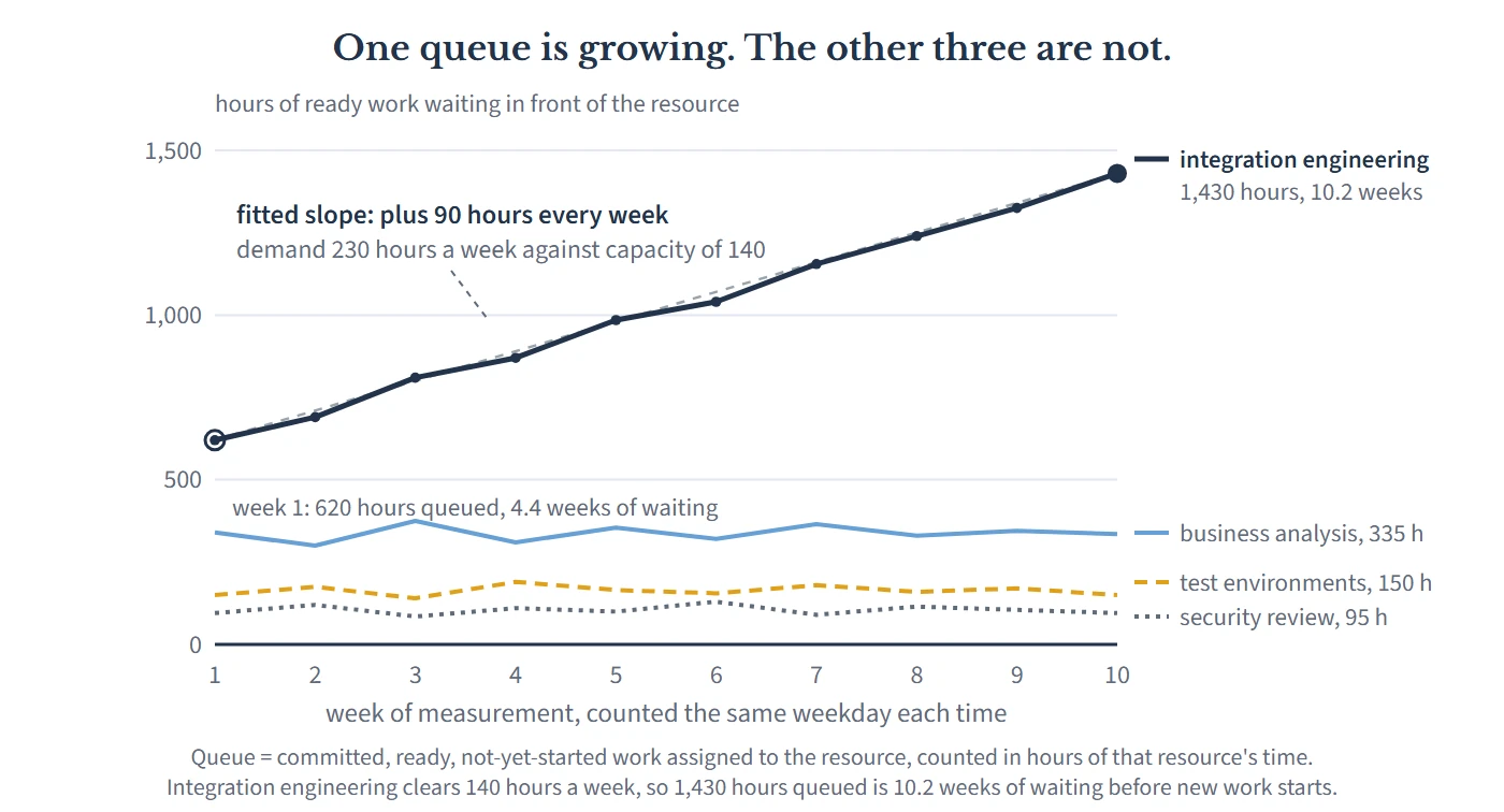
Business analysis, at 96% utilization, has a flat queue. That is not a contradiction, it is what a fully loaded resource in balance looks like: demand and capacity are the same number, and it clears work at the rate work arrives. It does have a real problem, which is that a resource running that hot with no reserve capacity turns every small piece of unevenness into a long wait, and that is a variability problem rather than a capacity problem. Hiring two analysts would have bought Calder some welcome protective capacity and not one week of portfolio throughput, because integration engineering would have gone on setting the pace, only with a bigger pile in front of it. That is the non-constraint trap, entered with good data and a straight face.
Integration engineering is 5 engineers who between them clear about 140 hours of queued work a week. The slope says work is arriving at about 230. Now read what those two numbers give you.
What does a slope tell you that a name cannot?
The size of the overload, in the unit you can act on. Demand exceeds capacity by 90 hours a week, which is 64% more work than the team can do. That is not a judgment or a mood, it is a subtraction. Utilization could never have produced it, because the number is made of hours nobody worked.
Today's wait, and last quarter's. A queue of 1,430 hours in front of a resource that clears 140 hours a week is 10.2 weeks of waiting before new work is so much as looked at. 10 weeks earlier the same division gave 4.4 weeks. Nobody at Calder decided to add nearly 6 weeks to every commitment the portfolio made, and nobody reported it, but that is what happened.
The rate at which your promises are degrading. Divide the slope by the completion rate: 90 divided by 140 is 0.64. Every week Calder runs this way adds about two thirds of a week, a little over three working days, to the wait facing everything not yet started. That sentence is the one to take to a steering board, because it turns an abstraction into a rate of loss that is still running while the meeting is happening.
The price. 12 of the 22 projects had integration work still queued. Each week of delay on an average Calder project costs about $18,000 in drag cost, the value the organization does not receive because a project finishes later than it could have: deferred savings, deferred premium income, or a commitment made against somebody else's date. The 10 weeks of unmanaged queue growth added 5.8 weeks of wait to each of those 12 projects, which is $104,400 a project and just over $1.25 million of value pushed out of the year. Divide that by the 810 hours the queue grew and you get roughly $1,500 of delayed value for every hour allowed onto that queue, which is the real price of an integration hour and the reason a new commitment should be priced before it is accepted rather than explained afterwards.
How much relief you now need, which is the number that hurts. There are two separate corrections here and they get conflated constantly. Stopping the growth takes 90 hours a week, permanently, either removed from demand or added to capacity. Clearing the 1,430 hours already queued, over a target of say 12 weeks, takes a further 119 hours a week on top of that. Total: 209 hours a week, against a team that produces 140. No hiring plan supplies one and a half times a specialist team inside a quarter, and adding people to a constraint makes it slower before it makes it faster, so the relief has to come from the demand side whether anyone likes it or not.
Notice the asymmetry in that last point, because it is the argument for measuring monthly rather than commissioning a study. The slope is a stable property of your intake: it was 90 hours a week in week 2 and 90 hours a week in week 10. The drain is not stable. It grows every week nobody looks. Had Calder run this in week 2, the correction would have been the same 90 hours a week of relief against a queue of 710 hours, roughly half the repair for an identical diagnosis. The cost of a late bottleneck analysis is not the analysis. It is that the bill for the remedy climbs steadily while you wait to be told something you could have measured on a whiteboard.
When more than one queue is growing
Two other readings are worth knowing, because both are common and both get misdiagnosed.
If every candidate queue has a positive slope, you do not have a constrained resource, you have an intake problem. No single resource can be the constraint when work accumulates everywhere at once. That pattern means the portfolio is accepting more work than the system as a whole can absorb, and the thing binding you is a policy rather than a team. That is good news, because a policy is cheaper to change than a specialist is to hire. The correction is a limit on work in flight, a hard cap on how many projects are allowed to be open at once.
If no queue is growing anywhere and delivery is still slow, your problem is not capacity and no amount of resourcing will touch it. The wait is in the handoffs: work sitting between steps with nobody's name on it, and decisions waiting for an authority to be available. That portfolio is not short of hours. It is short of flow.
Why single-project management is blind to this
Ask how Calder's queue grew for 10 weeks with nobody raising it, and the answer is not negligence. It is that nothing in single-project management is able to see a queue.
A project plan models work, not waiting. Calder's integration task appears on 12 different plans as a bar 2 or 3 weeks long, which is an honest estimate of the effort, and not one of those plans carries the 10 weeks of other people's work sitting in front of it, because that queue is not a property of any project. Each project manager meets the queue only as their own slip, which they then explain locally and correctly: the integration team was tied up, the environment was not ready, a supplier moved. 12 defensible local explanations, one shared cause, and no report anywhere that sums the column.
This is the Project Illusion, the assumption that a portfolio is a set of independent projects whose plans can be added together. Under that assumption a queue in front of a shared resource is not a managed object at all: it belongs to no project, has no owner, and appears on no plan. It is the largest single item of delay in most portfolios and it is structurally homeless. The only view that can see it is one that looks at the resource rather than at the projects, which is exactly what a bottleneck analysis is supposed to be, and exactly what a utilization table fails to deliver.
What to do instead
1. Put one page of slopes in front of your portfolio board every month. Four to eight candidate resources, a queue in hours, a fitted slope, a wait in weeks. Change nothing else at first. A number that gets published monthly behaves differently from a number produced during a crisis, because it makes the trend visible while the remedy is still cheap.
2. Report the wait in weeks, not the utilization in percent. "Integration engineering is at 91%" invites a shrug. "New work waits 10.2 weeks to start, and that wait grew by 5.8 weeks last quarter" is a sentence nobody can file. Percentages hide the thing you want a board to feel. Weeks do not.
3. Price the slope before you propose anything. Convert hours per week into weeks of added wait, then into drag cost across the projects actually queued, using your value per constrained resource hour if you have one and a defensible average project week if you do not. An overload described in hours gets negotiated. An overload described in dollars per week of inaction gets decided.
4. Separate stopping the growth from clearing the queue, with two numbers and two decisions. The first is a permanent change to intake or capacity. The second is a temporary surge with an end date. Most recovery plans fail because they attempt both with the funding for one, and land in the worst available position: a surge that ends, a slope that was never corrected, and a queue back where it started within a quarter.
5. Take the relief off the demand side first, and take it from the bottom of a ranked list. Deferring the lowest-returning work in the queue costs the least value per hour released, which is the point of ranking the portfolio by what it returns per constrained hour. Deferring whatever the least persuasive sponsor asked for is what happens when no ranking exists.
6. Require every new commitment to name the hours it adds to a named queue. One line on the approval paper: hours of the constrained resource consumed, and what this displaces. A gate that approves work without naming the displacement is not making a decision, it is recording an intention.
7. Re-run it, and expect the answer to move. When the correction works, the slope goes to zero and a different queue starts to grow, because relieving one constraint hands the role to the next-slowest necessary resource. That is the system telling you the fix landed. Treat a moving answer as the instrument working, not as evidence the first analysis was wrong. And if you have never done step one at all, start with how to find the resource that sets your delivery speed, then put the weekly count behind it.
The objection you are already forming
"Our data is nowhere near good enough for this. Our queue is not a real queue, it is a spreadsheet of intentions that gets reprioritized every fortnight, and half the hours in it are guesses."
Good, because that objection contains its own answer twice over.
On the data: look again at the arithmetic that mattered. Demand exceeded capacity by 64%. Suppose every hour estimate Calder used was wrong by 20% in the least convenient direction. The overload is still enormous, the wait is still months, and every decision above still goes the same way. A bottleneck analysis does not need accuracy, it needs consistency: the same definition, counted the same way, by the same person, every week. 10 wrong-but-consistent readings give you a sound slope, because a consistent error mostly cancels when you take a difference. One immaculately sourced snapshot gives you no slope at all, which is why a beautiful capacity study is worth less here than 4 numbers on a whiteboard for 2 months.
On reprioritization: shuffling the order of a queue does not change its size, and the slope is a measurement of size over time. Resequencing changes who waits, which is a real and important decision, and it changes the total wait not at all. If anything, frequent resequencing is corroborating evidence, because a queue short enough to be harmless is a queue nobody bothers to reorder. That fortnightly argument about whose work goes first is the queue making itself felt without ever being measured.
The deeper version of the objection is the honest one: that nobody really wants the number, because once it exists somebody has to say no to something. That is true, and it is the actual reason bottleneck analysis so often stops at a name. A name supports a recruitment case, which is a request for more. A slope supports a displacement decision, which is a request to do less, and the second is much harder to carry into a room even though it is the only one of the two that changes anything this year.
Your organization is paying the number whether it measures it or not. Calder paid $1.25 million over 10 weeks in delivery that simply arrived later, spread across 12 projects as 2 or 3 weeks each: small enough everywhere to be explained by something local, large enough in total to fund a sizeable piece of its change program. The queue was never hidden. It sat in a shared team's inbox the whole time, in plain view, unmeasured because the instrument everyone trusted was pointed at the resource instead of at what was waiting in front of it.
So count the pile, every week, in hours. A bottleneck analysis that returns a name tells you where to look. One that returns a slope tells you how much trouble you are in, how fast it is getting worse, and exactly what it would take to stop.

Leave a Reply